Below we have updated our 2006 white paper. While you can download the full 70+ page paper here, I’ve also chopped it up into a series of more digestible posts for the blog.
STEP 3 – GLOBAL TACTICAL ASSET ALLOCATION
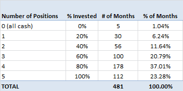
Given the ability of this very simplistic market-timing rule to add value to various asset classes, it is instructive to examine how the returns would look in the context of an investor’s portfolio. Here we introduce a version of the timing model we refer to as “Global Tactical Asset Allocation” or “GTAA”. GTAA consists of five global asset classes: US stocks, foreign stocks, bonds, real estate and commodities. The returns for a buy and hold allocation are referenced as “Buy & Hold” or “B&H” and are equally weighted across the five asset classes. The timing model also uses equal weightings and treats each asset class independently – it is either long the asset class or in cash with its 20% allocation of the funds. Figure 12 illustrates the percentage of months in which various numbers of asset classes were held. It is evident that the system keeps the investor 60%-100% invested the vast majority of the time (approximately ~80% of the time the portfolio is at least 60% invested). On average, the investor is 70% invested.
Figure 12: Percent of the Time Invested, 1973-2012
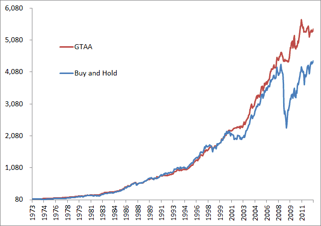
Figures 13 and 13b below present the results for the buying and holding of the five asset classes equal-weighted versus the timing portfolio. The buy and hold returns are quite respectable on a stand-alone basis and present evidence of the benefits of diversification.
Figure 13: Buy & Hold vs. Timing Model, 1973-2012, log scale
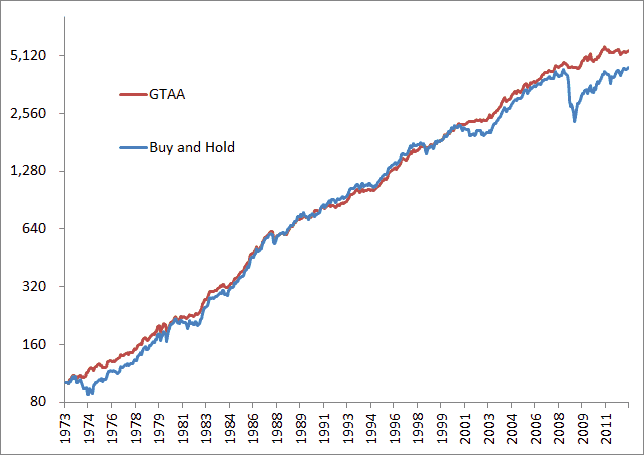
Figure 13b: Buy & Hold vs. Timing Model, 1973-2012, non-log scale
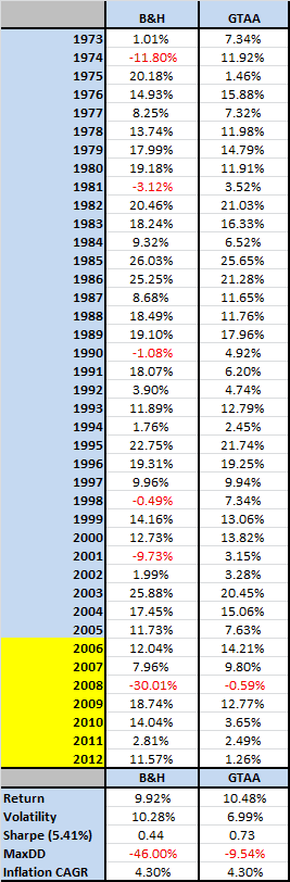
However, the additional advantages conferred by timing are striking. Timing results in a reduction of volatility to single-digit levels, as well as a single-digit maximum drawdown. Drawdown is reduced from 46% to less than 10%, and the investor would have only experienced one down year of less than -1% since inception in 1973. Figure 19 details the yearly returns, and post-2005 is highlighted as the out-of-sample period.
Figure 14: Yearly Returns for Buy & Hold vs. Timing Model, 1973-2012
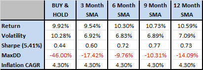
It is possible that Siegel (or others) have optimized the moving average by looking back over the period tested. As a check against optimization, and to show that using the 10-month SMA is not a unique solution, Figure 15 presents the stability of using various moving averages lengths ranging from 3 to 12 months. Calculation periods will perform differently in the future as cyclical and secular forces drive the return series, but all of the parameters below seem to work similarly for a long-term trend-following application.
Figure 15: Parameter Stability of Various Moving Average Lengths, Timing Model 1973-2012
While it is instructive to examine the model in various asset classes, the true test of a model is how it performs out of sample in real time. Since the paper was originally published in 2006 with results up to 2005, returns after 2005 should be seen as out of sample. Figure 16 illustrates the returns for B&H and timing portfolios.
Figure 16: Summary Annualized Returns for B&H vs. Timing Model, 2006-2012
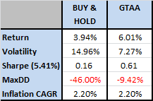
The model performed exactly as one would expect it to from historical data. Namely, even though it only outperformed in three out of seven years, it beat buy and hold by over two percentage points per year, with much less volatility and most importantly to many investors, lower drawdowns.