Below we have updated our 2006 white paper. While you can download the full 70+ page paper here, I’ve also chopped it up into a series of more digestible posts for the blog.
—-
STEP 2 – MANAGE YOUR RISK
There are a few criteria that are necessary for a model to be simple enough for investors to follow, and mechanical enough to remove emotion and subjective decision-making.
They are:
1. Simple, purely mechanical logic.
2. The same model and parameters for every asset class.
3. Price-based only.
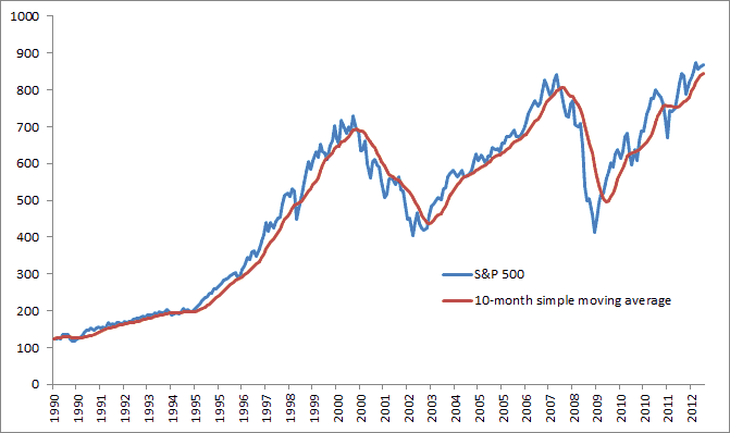
Moving-average-based trading systems are the simplest and most popular trend-following systems (see for example Taylor and Allen (1992) or Lui and Mole (1998)). For those unfamiliar with moving averages, they are a way to reduce noise. The example below shows the S&P 500 with a 10-month simple moving average (SMA).
Figure 6 – S&P 500 vs. 10-Month Simple Moving Average, 1990-2012
The most often cited long-term measure of trend in the technical analysis community is the 200-day simple moving average. In his 2008 book Stocks for the Long Run 5/E: The Definitive Guide to Financial Market Returns & Long-Term Investment Strategies, Jeremy Siegel investigates the use of the 200-day SMA in timing the Dow Jones Industrial Average (DJIA) from 1886 to 2006. His test bought the DJIA when it closed at least 1 percent above the 200-day moving average, and sold the DJIA and invested in Treasury bills when it closed at least 1 percent below the 200-day moving average.
He concludes that market timing improves the absolute and risk-adjusted returns over buying and holding the DJIA. Likewise, when all transaction costs are included (taxes, bid-ask spreads, commissions), the risk-adjusted returns are still higher when employing market timing, though timing falls short on an absolute return measure.
When applied to the NASDAQ Composite Index since 1972, the market timing system thoroughly outperforms buy-and hold, both on an absolute and risk-adjusted basis. Siegel finds that the timing model outperforms buy and hold by over 4% per year from 1972-2006 even when accounting for all costs, and with 25% less volatility. Unfortunately, Siegel does not report drawdown figures, which would have further demonstrated the superiority of the timing model. (Note: Siegel’s system is twice as active as the system presented in this paper, thus increasing the transaction costs). Sigel is updating the book with a 2013 edition, and we look forward to see the results including the 2006-2012 period.
It is possible that Siegel already optimized the moving average by looking back over the period in which it is then tested. To alleviate fears of data mining, the approach will be examined across various parameters and other markets to test for validity.
The system is as follows:
BUY RULE
Buy when monthly price > 10-month SMA.
SELL RULE
Sell and move to cash when monthly price < 10-month SMA.
1. All entry and exit prices are on the day of the signal at the close. The model is only updated once a month on the last day of the month. Price fluctuations during the rest of the month are ignored.
2. All data series are total return series including dividends, updated monthly.
3. Cash returns are estimated with 90-day Treasury bills, and margin rates (for leveraged models to be discussed later) are estimated with the broker call rate.
4. Taxes, commissions, and slippage are excluded (see the Practical Considerations section later in the paper).
S&P 500 FROM 1901 – 2012
To demonstrate the logic and characteristics of the timing system, we test the S&P 500 back to 1901. Total return series is provided by Global Financial Data and results pre-1971 are constructed by GFD. Data from 1901-1971 uses the Standard and Poor’s Composite Price Index and dividend yields supplied by the Cowles Commission and from S&P.
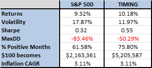
Figure 7 presents the annualized returns for the S&P 500 and the timing method for the past 100+ years. A cursory glance at the results reveals that the timing solution improved compounded returns while reducing risk, all while being invested in the market approximately 70% of the time and making less than one round-trip trade per year. (Volatility is measured as the annualized standard deviation of monthly returns.)
Figure 7: S&P 500 Total Returns vs. Timing Total Returns (1901-2012)
The timing system achieves these superior results while underperforming the index in roughly half of all years since 1901. One of the reasons for the overall outperformance is the lower volatility of the timing system. It is an established fact that high volatility diminishes compound returns. This principle can be illustrated by comparing average returns with compounded returns (the returns an investor would actually realize.) The average return for the S&P 500 since 1901 was 11.26%, while timing the S&P 500 returned 11.22%. However, the compounded returns for the two are 9.32% and 10.18%, respectively. Notice that the buy and hold crowd takes a hit of nearly 200 basis points from the effects of volatility, while timing suffers a smaller decline of around 100 basis points. Ed Easterling has a good discussion of these “volatility gremlins” in John Mauldin’s 2006 book, Just One Thing: Twelve of the World’s Best Investors Reveal the One Strategy You Can’t Overlook.
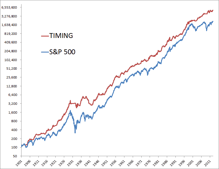
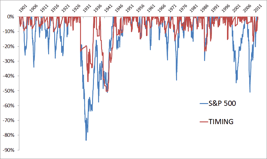
Figure 8 shows the superiority of the timing model over the past century, largely avoiding the significant bear markets of the 1930s and 2000s. Figure 8b shows that timing would not have left the investor completely unscathed from the late 1920s early 1930s bear market, but it would have reduced the drawdown from a catastrophic 83.66% to a more manageable 42.24%.
Figure 8: S&P 500 Total Returns vs. Timing Total Returns (1901-2012)
Figure 8b: S&P 500 Drawdowns vs. Timing Drawdowns (1901-2012)
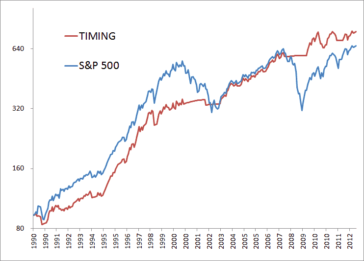
Figure 9 is charted on a non-log scale to detail the differences in the two equity curves. Examining the most recent 22 years, a few features of the timing model stand out. First, a trend-following model can underperform buy and hold during a roaring bull market similar to the U.S. equity markets in the 1990s. On the flip side, the timing model can avoid lengthy and protracted bear markets. Consequently, the value added by timing is evident only over the course of entire business cycles.
For example, the timing model exits a long position in October of 2000, thus avoiding two of the three consecutive years of losses, and its 16.52% drawdown is much shallower than the 44.73% setback suffered by buy-and-hold investors. The timing model again exited the S&P 500 on December 31, 2007 and avoided the entire bear market of 2008-2009 and the 50.95% drawdown.
Figure 9: S&P 500 Total Returns vs. Timing Total Returns (1990-2012)
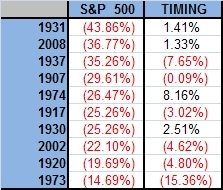
A glance at Figure 10 presents the ten worst years for the S&P 500 for the past century, and the corresponding returns for the timing system. It is immediately obvious that the two do not move in lockstep. In fact, the correlation between negative years for the S&P 500 and the timing model is approximately -0.38, while the correlation for positive years is approximately 0.83. This reflects the ability of the timing model to stay long in up markets while exiting the long position during down markets.
Figure 10: S&P 500 Ten Worst Years vs. Timing, 1900-2012
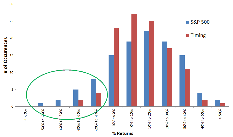
Figure 11 gives a good pictorial description of the results of the trend-following system applied to the S&P 500. The timing system has fewer occurrences of both large gains and large losses, with correspondingly higher occurrences of small gains and losses. Essentially, the system is a model that signals when an investor should be long a riskier asset class with potential upside, and when to be out and sitting in cash. It is this move to a lower-volatility asset class (T-bills) that drops the overall risk and drawdown of the portfolio. Most importantly, it avoids the far left tail of big negative losses.
Figure 11: Yearly Return Distribution, S&P 500 and Timing 1900-2012
Appendix B breaks down the returns down by decade for the S&P 500 and the timing model. While the timing model outperforms in about half of all decades on an absolute basis, it improves risk-adjusted returns in about two-thirds of all decades and improves drawdown in all but two decades. Another interesting observation is the wide variance in Sharpe ratios per decade for buy and hold, ranging from -0.23 to 1.44. The past decade has seen compound returns of -0.94% per year for buy and hold while the 1950s saw returns of 19% per year.

